Example in Renew
Renew Models for RobotOPN and SpecOPN
Let us recall the formal notation of the sets of regions of interest
$\mathcal{Y} = {y_1, y_2, \dots y_{|Y|}}$, respectively of atomic propositions
$\mathcal{B} = {b_1, b_2, \dots b_{|B|}}$.
For a simpler visualization in the Renew simulator, the notations are redefined to eliminate the subscripts. For example, the formal notation of atomic propositions $\mathcal{B}$ for the set of regions
$\mathcal{Y} = {y_1,y_2,y_3,y_4}$ (Figure 1) is replaced by the set ${a,b,c,w}$ in exactly this order, with $w$ assigned to the free space $y_4$.
Additionally, the symbols $\neg$ and $\wedge$ are replaced in Renew with the syntax ! and ,, respectively. The True value returned by the associated Büchi automaton of the co-safe LTL formula is represented in the tool by 1.
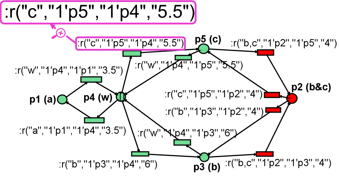
Figure 1. Examples of the RobotOPN models in Renew: Robots $r_1$ qpn_robot and $r_2$ qpn_robot_2 are free to move throughout the workspace. Robot $r_3$ is prohibited from entering the overlapping area between $y_2$ and $y_3$ (excluding the red places and transitions).
Firstly, Figure 1 portrays the design of a $RobotOPN$ representation, considering the environment described in Figure 1. Specifically, the workspace contains a set of 3 regions of interest, two of them being overlapped $y_2 \wedge y_3$.
- Robots $r_1$ and $r_2$ move freely.
- Robot $r_3$ is not allowed to enter the overlapped region.
Thus, the place $p_2$ modeling the overlaid area together with the input and output transitions are highlighted in red. In other words, the $RobotOPN$ model for $r_3$ includes only the places and transitions colored in green, while $r_1$ and $r_2$ are associated with a Petri net modeled by all the places and transitions illustrated in the figure.
Each transition is labeled (magenta color). For instance, the label (c,1'p5,1'p4, ...) corresponds to the information required for synchronization, used by the GEF:
- The robot occupies one unit in the region labeled with $c$ (modeled by $p5$).
- It frees its position from the free space $w$ (modeled by $p4$).
Thus, the atomic proposition for $c$ is evaluated as True. The last parameter in the label represents additional robot information, e.g., the movement time. In this example, the robot needs 5.5 time units to move from $p4$ to $p5$, assuming constant velocity.
Remark. In the implementation, there are two Renew models for these two types of robots:
- Since $r_1$ and $r_2$ have the same spatial constraints, a single RobotOPN model is sufficient, including all 5 places.
- For $r_3$, the RobotOPN model includes only 4 places, excluding the overlapped region modeled by $p2$.
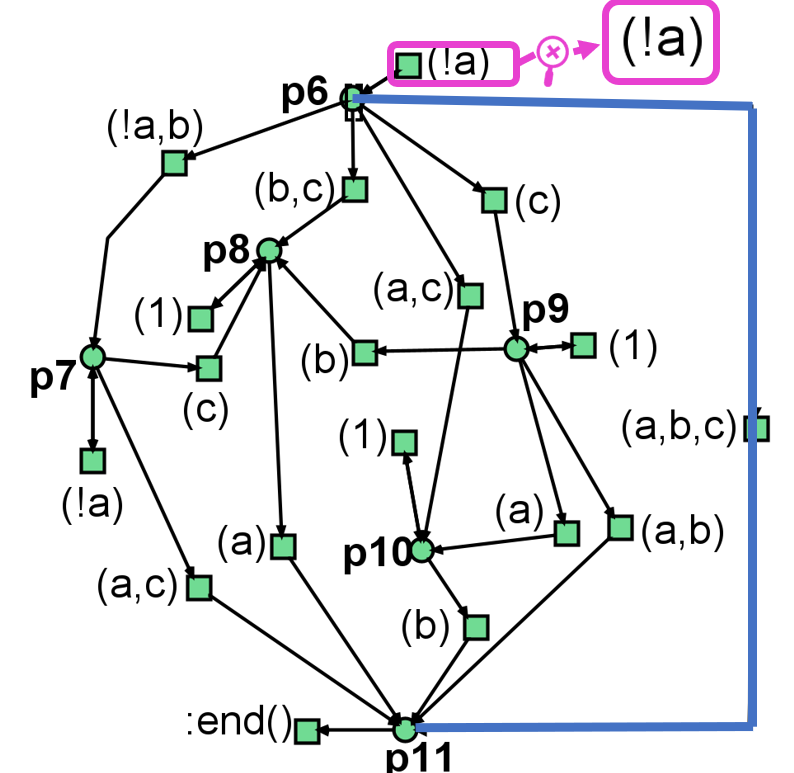
Figure 2. Renew SpecOPN model for the LTL formula
$\varphi= \diamondsuit b_1 \wedge \diamondsuit b_2 \wedge \diamondsuit b_3 \wedge \left(\neg b_1~\mathcal{U}~b_3\right)$.
Figure 2 illustrates the SpecOPN model in Renew, associated with the mission
$\varphi= \diamondsuit b_1 \wedge \diamondsuit b_2 \wedge \diamondsuit b_3 \wedge \left(\neg b_1~\mathcal{U}~b_3\right)$.
- Transition labels (magenta) indicate atomic propositions.
- For example,
(!a)expresses the negation of atomic proposition $b_1$ associated with region $y_1$. - The blue color shows the run returned by Renew after 100 simulations, representing the shortest path of the robotic team.
The place :end() models the final state: a token in place $p11$ means the mission is achieved.
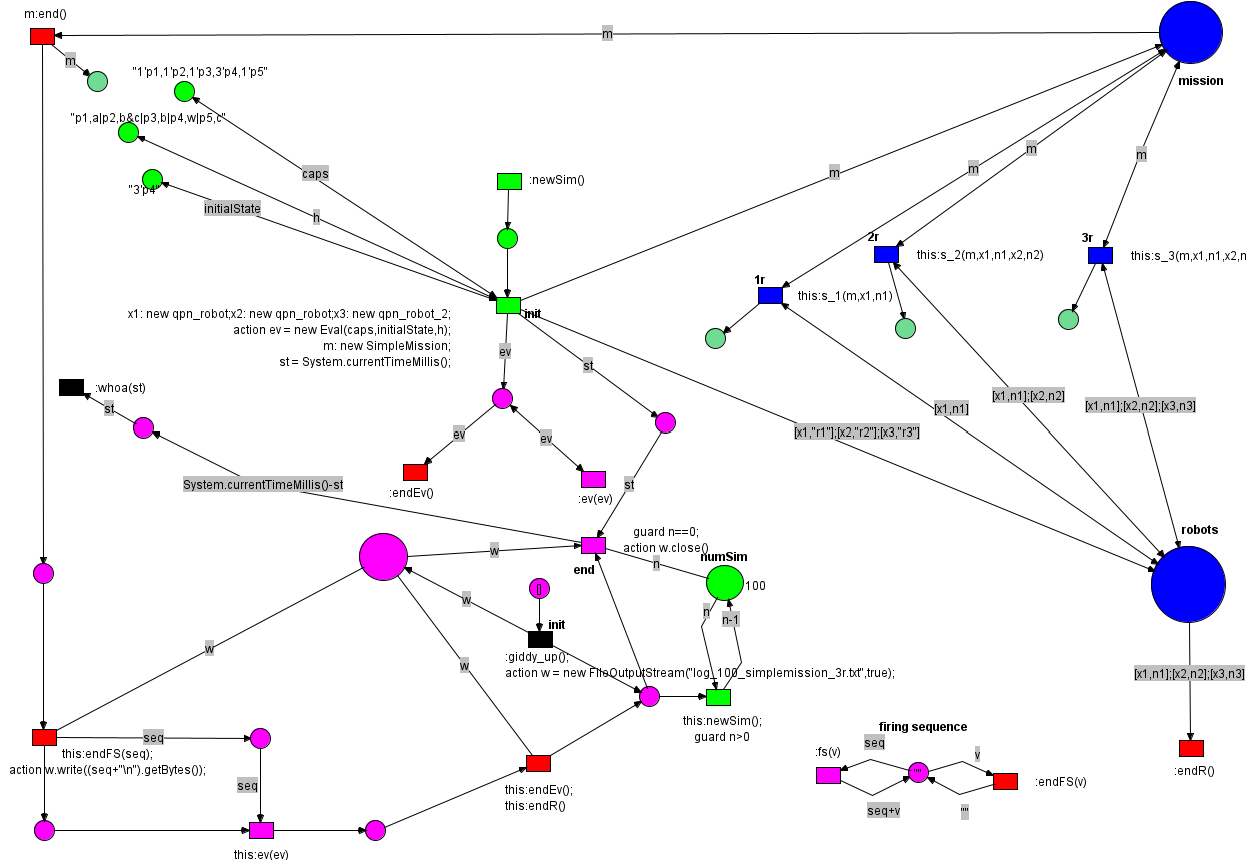
Figure 3. Example of the High-Level robotic team Petri net model in Renew.
Figure 3 portrays the main file representing the High-Level robotic team Petri net framework under the Nets-within-Nets paradigm.
- The blue places show the system net:
missioncontains as a token the $SpecOPN$ model.robotscontains three tokens referencing the $RobotOPN$ models.
- Blue transitions are added for each robot.
- Other colors:
- Green = simulation inputs (max capacity, atomic proposition mapping, initial positions).
- Red = finalizing simulation.
- Pink = process results (shortest path, run time).
For instance, on the top left, three green places define:
- Maximum capacity per place (e.g., 3 robots in free space $w$).
- Association between places and atomic propositions (e.g., $p_4$ models $w$).
- Initial robot positions (all robots starting in free space).
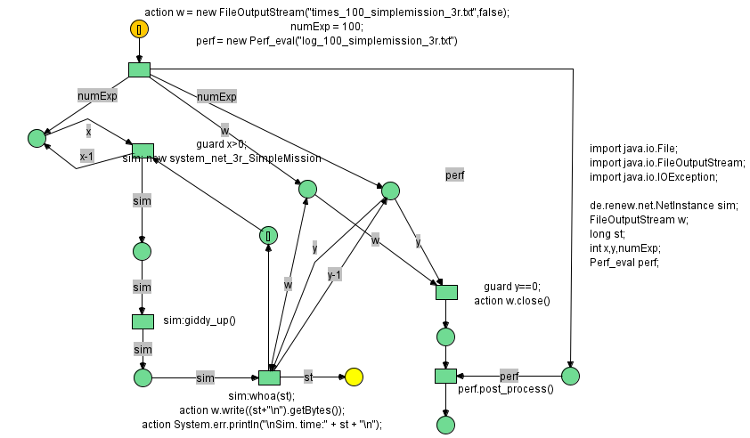
Figure 4. Example of the execute_experiment net in Renew.
To run the simulations, another net is modeled in Renew, called execute_experiment. This net encapsulates data about the simulation:
- Number of simulations per experiment.
- Names of the
.txtfiles storing paths. -
Total run time (ms).
- Orange = input place.
- Yellow = end place.
When the token reaches the yellow place, the experiment ends and the results are saved.
Information on the files
Simulation information :
- At all times, you can observe the state of the robots nets by right-clicking the number contained by the Master Net place and double-clicking on one robot.
- You can simulate by choosing the fired place. After having fired “init”, you can double click on a transition si and choose what transition to fire.
- The system will be executed as many times as the initial marking of place “numSim”.
- All the traces will be accumulated to the file named “log.txt”.
- Besides storing in “log.txt” the solutions found, the “best” one will be in place named “bestSol”. Being initially “”, each time a new solution is obtained, it is compared with the current best, by means of the function “select_best” in the class “Eval”. In its current version, “best” means “shorter” in terms of number of chars, but this is so just to check the feasability. The function could/should be much more sophisticated